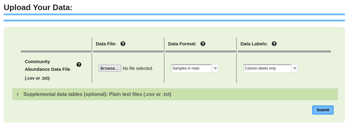
1 Data Upload and Processing

The initial step entails uploading community abundance data. Within this tutorial, we showcase WEGAN's functionalities using example datasets including Aravo, BCI, Dune, Tussock, Ursine Aquatic Prey and Varespec. Data should be uploaded as a tab-delimited (.txt) or comma-separated values file (.csv). Several different data types are required by each module with community abundance data essential to all modules. Clustering and Classification, Correlation, Dispersal and Statistics can also include environmental data; Ordination, Plotting and Taxonomy can also include environmental and/or taxonomic data and Diversity can also include environmental and/or trait data. Community abundance data is best configured with the species in columns and sites in rows and environmental data is best configured with variables in columns and sites matching the community abundance data in rows. Trait data is best configured with trait variables in columns and species matching the community abundance data in rows and taxonomic data is best configured with taxonomic variables (genus, family, etc.) in columns and species matching community abundance data in rows. Select the orientation for samples (sites in rows or columns) and whether to use column names/row names. Community abundance data feature names are designed to be species but can be any taxonomic level or any other variable appropriate for your data analysis.

1.1 Data Upload

Follow the provided instructions to upload custom data. Refer to the user interface screenshot (Figure 1.1.1) for updating the custom data.

Figure 1.1.1: Web page for data uploading in the modules.

1. Upload Data: Click the "Browse" button in the "Data File" column to upload custom data (.csv or .txt files). For detailed instructions, hover over the question mark icons next to input fields.

2. Specify Data Format: Choose the format of the uploaded community abundance data from the dropdown in the "Data Format" column.

3. Specify Data Labels: Ensure accurate representation by selecting appropriate data labels from the dropdown in the "Data Labels" column.

4. Click the “Submit” button to proceed to the following steps.

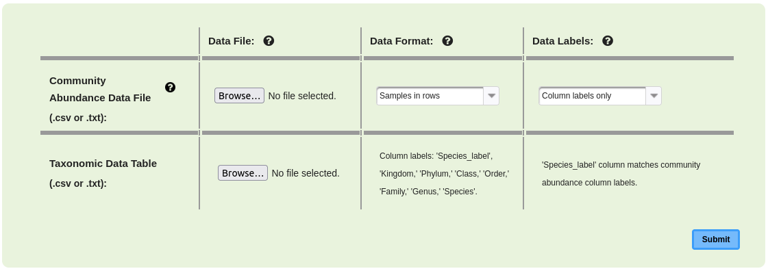
The taxonomy module requires additional taxonomy data (Figure 1.1.2).

Figure 1.1.2: Web page for data uploading in the Taxonomy module.

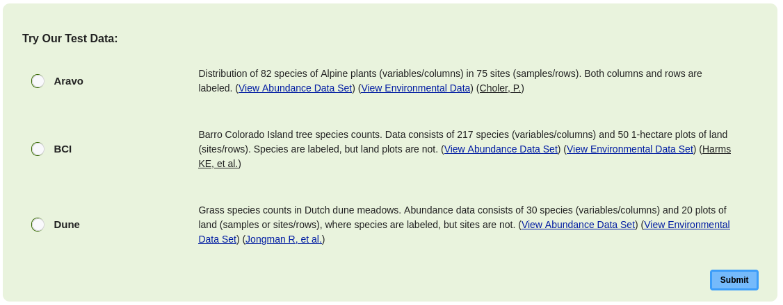
1.1.1 Try Our Test Data

Alternatively, users can utilize example data provided within the Cluster and Classification module.

In the panel labeled "Try Our Test Data" (Figure 1.1.3, example from the Cluster and Classification module), three example datasets are available: Aravo (Distribution of 82 species of Alpine plants), BCI Environmental Data (Environmental data for tree species counts from Barro Colorado Island), and Dune (Grass species counts in Dutch dune meadows).Users can select their preferred dataset by clicking the radio button next to it and proceed to the next steps. Detailed documentation regarding the data format and labels is provided beside the radio buttons. Additionally, users can view and download the dataset by clicking on the hyperlink following the description.

1. Choose the desired example data: Click one radio button for the respective data.

2. Click the “Submit” button to proceed to the following steps.

Figure 1.1.3: Panel displaying example data on the data upload page for the Clustering and Classification module.

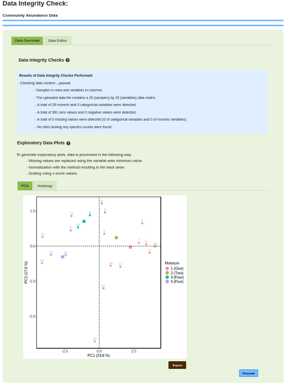
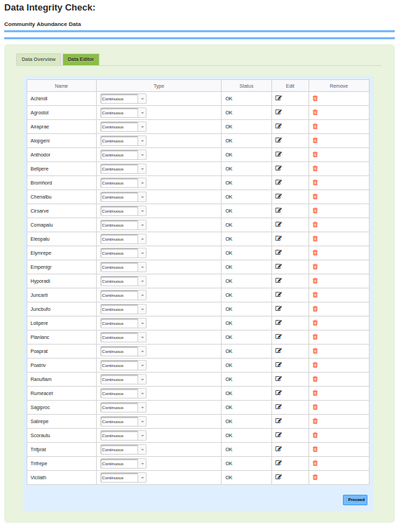
1.2 Data Processing

1.2.1 Integrity Check of Data

After uploading data, integrity checks are conducted on statistical data. In the navigation tree, 'Data Check' is highlighted under 'Processing'. If data meets integrity criteria (Figure 1.2.1), users can proceed; if not, detailed errors are shown in the result panel, prompting users to adjust and reload their data. The upper panel (green) displays data integrity criteria (presence of missing values and checking sample and variable labels), while the lower panel (blue) shows dynamic results from uploaded data. The blue panel contains the data you have uploaded; identifying the name of the species, the type of data it contains (Continuous, Categorical, Ordinal), whether or not the species passes the integrity check, and buttons to either edit individual entries or remove the species.

The data overview tab shows the data integrity checks and exploratory data plots. The data integrity check shows if the data meets the integrity criteria. The exploratory data plots show the data in graphical form. Two plotting options, PCA and heatmap, can be used to access and explore data before analysis.

The data editor tab can be used to check the status of individual variables, change the type of data, edit the metadata, or delete variables (Figure 1.2.2).

Figure 1.2.1: Web Page for Clustering and Classification data integrity check.

Figure 1.2.2: Web Page for data editor.

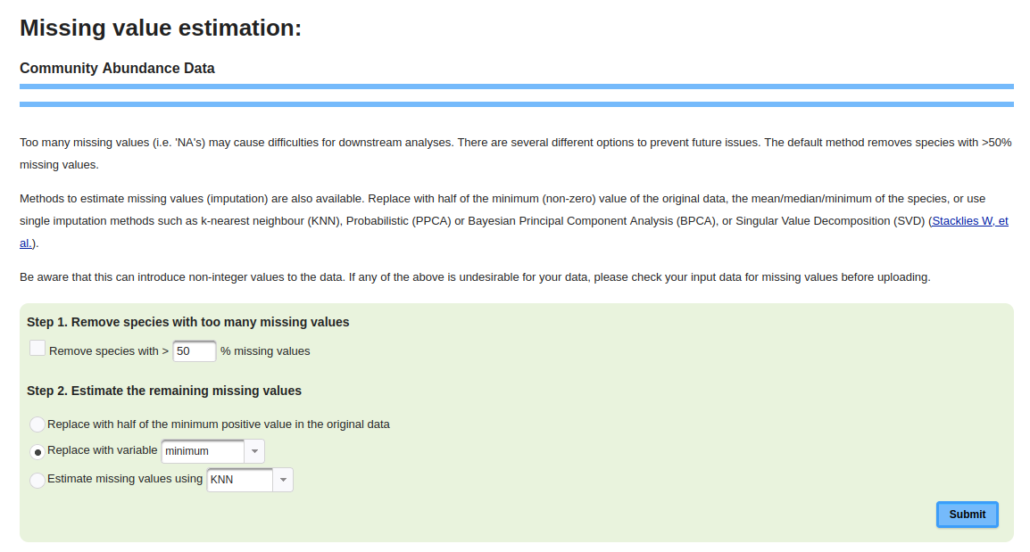
1.2.2 Missing Data Values

If missing data were detected, the link to the Missing Value Estimation page becomes enabled. This page provides two steps to deal with missing values.

Step 1 is to remove species that have some percentage of their data missing. This percentage is configurable by the user, allowing them to customize which species can be removed (Figure 1.2.3).

Step 2 involves selecting a process to replace the remaining missing values using one of the radio buttons and menus (Figure 1.2.3). For radio button 2, the menu may be changed from minimum to mean or to median. For radio button 3, the menu may be changed to k-nearest neighbor (KNN), Probabilistic (PPCA), Bayesian Principal Component Analysis (BPCA), or Singular Value Decomposition (SVD).

Figure 1.2.3: Missing values adjustment.

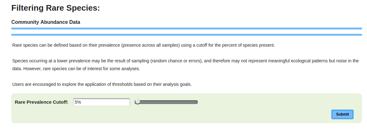
1.2.3 Filtering of Data

In the Correlation module, rare species can be defined based on their prevalence (presence across all samples) using a cutoff for the percent of species present.

Species occurring at a lower prevalence may be the result of sampling (random chance or errors), and therefore may not represent meaningful ecological patterns but noise in the data. However, rare species can be of interest for some analyses.

Users are encouraged to explore the application of thresholds based on their analysis goals. (Figure 1.2.4).

Figure 1.2.4: Web page for data filtering of uploaded Correlation data.

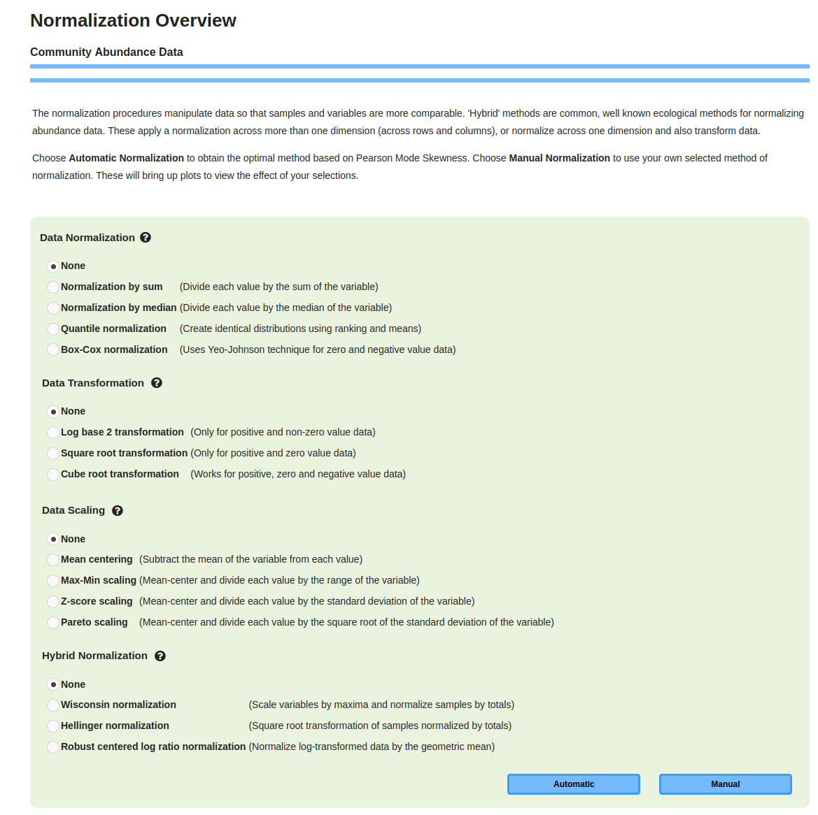
1.2.4 Normalization of Data

Normalization procedures manipulate data so that samples and variables are more comparable. Choose "Automatic Normalization" to obtain the optimal normalization based on Pearson Mode Skewness. Choose "Manual Normalization" to use your selected method of normalization. These options will bring up plots to view the effect of your selections. The green panel presents various method options for normalization and scaling (Figure 1.2.5).

Figure 1.2.5: Web page for Normalization processing.

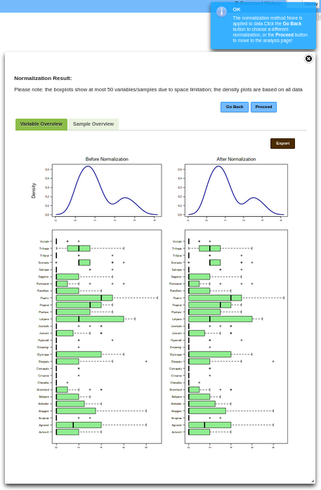
Upon normalization, users can visualize the data distribution before and after the process. When the "Automatic Normalization" or "Manual Normalization" button is active, a dialog window titled "Normalization Result" appears. The box plots show at most 50 variables/samples due to space limitation; the density plots are based on all data. Users can proceed to the next step by clicking "Proceed" if satisfied or return to the method menu page by clicking "Go Back" if unsatisfied (Figure 1.2.6).

Figure 1.2.6: Dialog window for normalization results.

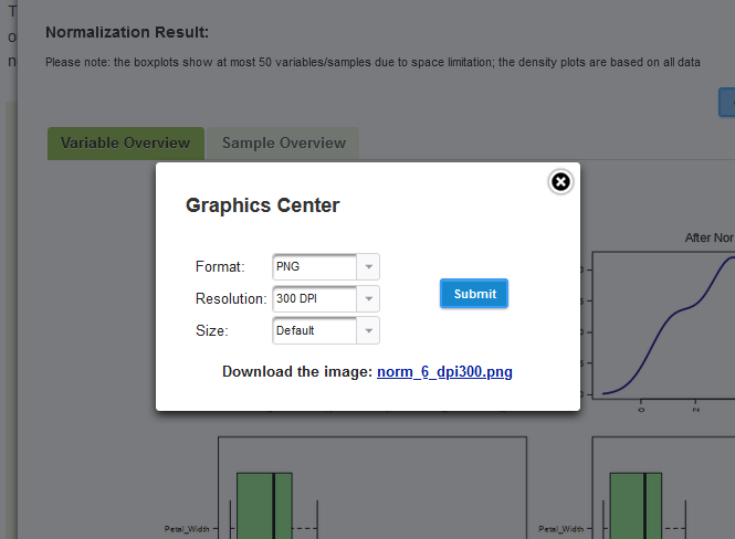
In the "Normalization Result" dialog window, users can explore data distribution plots for variables and samples by selecting the "Variable Overview" and "Sample Overview" tabs, respectively. To download distribution plots, users can click the "Export" button. This opens a dialog box titled "Graphics Center" allowing adjustments to the "Format," "Resolution," and "Size" of the plots. After confirming these parameters, clicking "Submit" generates a hyperlink for download (Figure 1.2.7). Users can click “Proceed” to finish data normalization and jump into the main page of the desired module.

Figure 1.2.7: Dialog box for graphics center for export.